| Home | Software | Example Cases | Contact | Bio |
NASA TM 2001 210652, Body Alone
OK, time to compare to data. The following example compares PANAIR and AT CFD Euler and Navier Stokes (laminar and Spalart-Allmaras (SA-noft2)) results to the body alone data provided in NASA TM 2001 210652 (ntrs.nasa.gov).
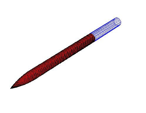
The PANAIR model of the geometry is shown in the figure below.
The body alone configuration is an ogive-cylinder with a diameter of 3.0 inches, a nose length of 9.0 inches, and a total body length (nose tip to base) of 36.0 inches. The moment center is located 21.0 inches from the nose tip. The reference length is equal to the body diameter (3.0 inches) and the reference area is equal to the cross sectional area (π×1.52). The data covers a Mach range of 0.60 to 3.95. The data for Mach numbers up to and including 1.20 were obtained from the Langley 8 ft. Transonic Pressure Tunnel (8-FT TPT). The remaining Mach numbers were obtained from the Langley Unitary Plan Wind Tunnel (UPWT). A transition strip of grit was located about 1.2 inches aft of the "nose" of the axisymmetric body. I'm assuming that "nose" refers to the nose tip.
Shown below is a table with the Reynolds number per foot vs. wind tunnel Mach number.
| Mach | Re/ft |
| 0.60 | 2.7e6 |
| 0.90 | 2.0e6 |
| 1.20 | 1.7e6 |
| 1.60 | 2.0e6 |
| 2.00 | 2.0e6 |
| 2.30 | 2.0e6 |
| 2.96 | 2.0e6 |
| 3.95 | 2.0e6 |
The figure below compares the axial force coefficient (CX) results from PANAIR and AT_CFD Euler and Navier Stokes to data in TM 2001 210652.
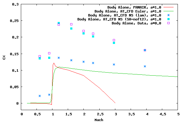
The base pressure has been neglected, i.e. it has been set to p∞ for the results and data. The analytic results were calculated at an angle of attack of one degree. The grid for the AT CFD computations does not include the base, i.e. the body extends well past the base, but the body load integration ends at the base. The boundary conditions for the AT CFD computations are such that the outer far field (K=kmax-1) is set to freestream, the back far field (I=imax-1) is set to zero gradient, the forward face (I=0) is set to a 2nd order extrapolated axis, and the body (K=0) is set to 1st order extrapolation. The J boundary conditions are set to symmetric since ½ of the grid is being modeled.
From the figure it can be seen that the axial forces predicted by PANAIR and Euler are essentially zero at subsonic speeds. At supersonic speeds the PANAIR results are in good agreement to the Euler results up to Mach 1.5. Since viscous and skin friction modeling is absent, both the PANAIR and Euler results compare poorly to data. It can also be seen that the laminar Navier Stokes results compare poorly. This is a consequence of the flow being turbulent over the length of the body. For a flat plate with a ReL of 8.1e6 (2.7e6×3.0 ft.), the ratio of drag for smooth turbulent flow to laminar flow is about 6.8. The Spalart-Allmaras (SA-noft2) results compare much better.
The figure below compares the normal force coefficient (CZ) results from PANAIR and AT_CFD Euler and Navier Stokes results to data in TM 2001 210652.
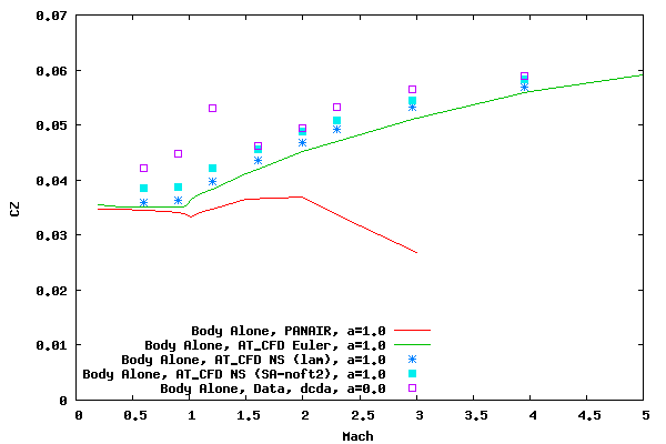
In the figure above, the analytic results are calculated at one degree angle of attack. However, the data is shown by means of the normal force coefficient slope with respect to the angle of attack (dCN/dα) where the angle of attack is measured in degrees. The slope is taken at zero degrees angle of attack.
From the plot above it can be seen that PANAIR for a body alone does not compare well to data or the Euler results for supersonic values. The PANAIR trend for CZ is similar to those presented in the 2 and 4 caliber examples. It should be noted, if fins or wings were introduced PANAIR would compare better for the supersonic Mach numbers since the normal force of the wing (which is better predicted by PANAIR) would dominate the loads. This can be seen in the TM 2001 210652, w. Fin 11 example.
In general, the Euler normal force coefficient results compare OK to data. Some difference is attributed to the rotation of the skin friction vector due to the angle of attack. For example, at Mach 0.6 the wind tunnel axial coefficient is about 0.142. Multiplying this value by sin(1.0) results, approximately, in 0.0025, which is similar to the average difference between data and Euler results.
Since the Navier Stokes results take into account the skin friction contribution to normal force, they compare better than Euler to wind tunnel. Though, at subsonic and transonic speeds, the wind tunnel results still differ from the Navier Stokes results. The difference may be attributed to wind tunnel effects and the lack of modeling a base and sting.
The figure below compares the pitching moment coefficient (CZ) results from PANAIR and AT CFD Euler and Navier Stokes to data in TM 2001 210652.
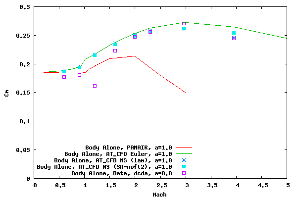
In the figure above, the analytic results are calculated at one degree angle of attack. However, the data is shown by means of the pitching moment coefficient slope with respect to the angle of attack (dCm/α) where the angle of attack is measured in degrees. The slope is taken at zero degrees angle of attack.
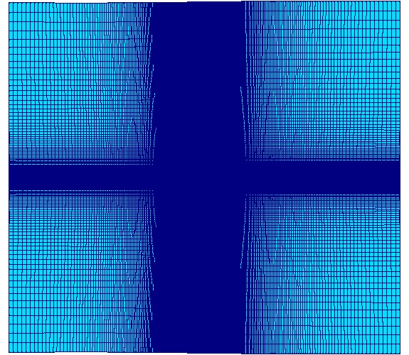
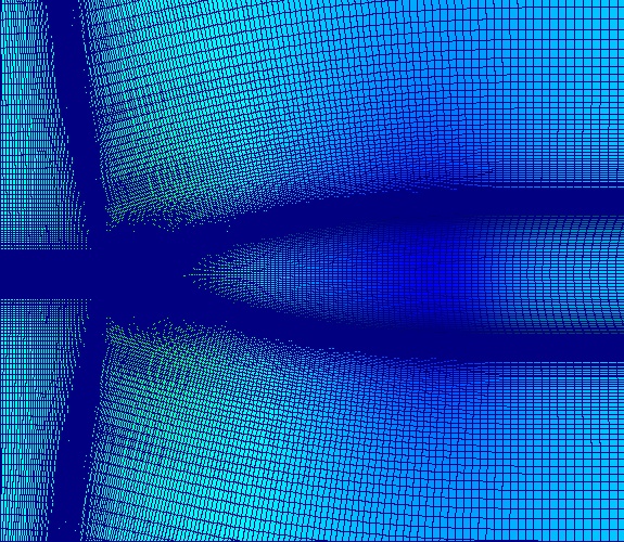
The figures below show various p/p∞solution and grid snapshots for the Mach 0.90 α 1.0 degree AT CFD Navier Stokes (laminar) case.
Solution in vicinity of geometry. The total number of grid points is approximately 6.14 million.
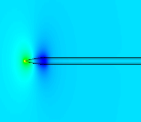
Solution in vicinity of nose.
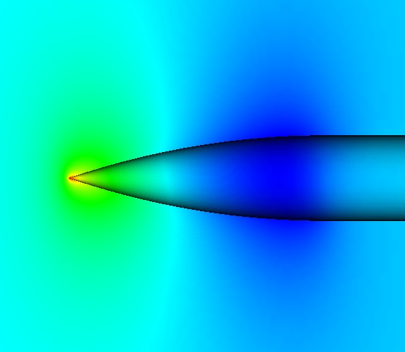
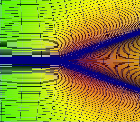
Solution and grid in vicinity of nose.
Solution and grid in vicinity of nose tip.
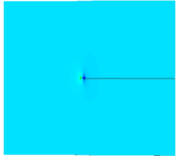
Farfield solution.
Farfield solution and grid.