This is my analysis of the classic Pulliam and Chaussee's diagonal implicit approximate-factorization algorithm1 (DADI). I undertook the analysis to understand why an axisymmetric Ogive Cylinder case of mine was experiencing difficulty converging, even at low CFL numbers. The code I am using is my own AT CFD code which is a steady state compressible finite difference Navier-Stokes solver using local time stepping and the Pulliam and Chaussee's diagonal implicit approximate-factorization algorithm. The code is first order accurate in time and second order accurate spatially.
During the course of this analysis I develop a modification term to the classical DADI to convert the factored DADI differencing terms back to the Jacobian matrix differencing terms of the Beam and Warming ADI method. At the moment I am calling my version the MDADI method. Since the modification terms bring the DADI terms back to the Jacobian matrix terms, I do not consider the MDADI method an enhancement over the Beam and Warming method. However, I use the MDADI terms to shed light on the DADI method and to help with debugging. The terms may also help reduce computational effort and to spatially fuse the DADI method with the ADI method. In other words, some portions of the grid could use ADI and others use DADI.
During the course of this analysis I determine a metric which may help determine when the DADI or ADI method should be used. The metric is then dissected to give an idea of when an axisymmetric grid using the DADI approach may run into difficulties.
Finally, the axisymmetric Ogive-Cylinder case is used to illustrate some of the points made.
To date, I have not seen such an analysis as this. Which is odd since the DADI method is used in many codes, such as OVERFLOW2. If someone sees such an analysis, please email me and let me know.
Executive Summary
When all is said and done, my problem boils down to the neglect of terms in the product rule, as specified in reference 1.
Equation (25) of reference 1 states that the difference (r) between the ADI and DADI is
r=hδx(Xn)ΛnA(X-1)nΔqn+O(hδqnΔxp)
As stated in reference 1, "The error introduced by the diagonalization is first order in time." The concept of "time" accuracy holds true even for codes which march forward in time towards steady state using a local time stepping. Except, in this case, time is not physical time. Since the error term is on the order of the time accuracy of AT CFD, AT CFD has difficulty converging.
The focus of the error is on the δx(Xn) term. In reference 1 the term is presented for a 1D problem. To get a better idea of the error, the term will be presented for a 3D problem and expanded out in the η direction.
δη(Xn)=∂k(Xn)δηk+∂qn(Xn)δηqn
Where k is the unit normal vector for the cell η face. (Note: for the rest of the analysis khat is used for the unit normal instead of k)
Therefore, it is clear that the error term is dependent on the change in direction of the face normal vector along with the change in flow values. In general, neglecting these terms does not seem to be a problem. However, as the axis for an axisymmetric case is approached, ηx gets large and this seems to amplify the error term. In other words, the error term is a function of the distance from the axis, i.e. the radius at which the point is located. Also, the error is not confined to a small region of the grid. It extends all along the axis. Therefore, the error has a chance to build up faster than it can be propagated away.
Derivation of MDADI Equations
The derivation starts with Pulliam and Chaussee's implementation of the standard DADI method before the eigenvector matrices have been factored outside of the differencing operator. This is equation (11) from reference 1.
[I + hδξ(TξΛξT-1ξ)][I + hδη(TηΛηT-1η)][I + hδζ(TζΛζT-1ζ)]Δqhatn = Rhatn (eq. 1)
As an example, the second delta term will be worked with.
h[δη(TηΛηTη-1qhatζn)]
The term qhatζn represents the remaining factored term, i.e. the &zeta factored term. From here on out I am going to drop the η subscript.
Next, the product rule will be used on the delta term.
h[δ(TΛT-1qhatζn)]=h[δ(T)ΛT-1qhatζn]+h[Tδ(ΛT-1qhatζn)]
The error term (equation (25) of reference 1) is the first term on the right of the equals sign. As in reference 1, the error term is labeled 'r'.
r=h[δ(T)ΛT-1qhatζn] (eq. 2)
At this point it should be noted that the error term is a first order function of the time step. As the time step becomes large, the time step will cancel with the time step operator in the Rhatn term of equation 1 (which in the case of AT CFD is first order). Therefore, the error term, or convergence modification term, becomes independent of the time step as the time step increases in size.
Next the partial derivative of T will be taken with respect to the unit normal vector (khat) and the flow values.
r=h[(∂khat(T)δkhat+∂q(T)δq)ΛT-1qhatζn]
Next T and T-1qhatζn will be factored out.
r=Th[(T-1∂khat(T)δkhat+T-1∂q(T)δq)Λ]T-1qhatζn
This equation will be visually simplified to
r=Th[(P+S)Λ]T-1qhatζn (eq. 3)
Where P=T-1∂khat(T)δkhat and S=T-1∂q(T)δq
In the formation of equation (18a) of reference 1, the T and T-1qhatζn will be pulled out. Therefore the focus will be on the term between these two values. This will be labeled rhat.
rhat=h[P+S]Λ (eq. 4)
Next, the P term will be looked at. This represents the change in the T matrix while leaving the flow values constant.
P=T-1∂khat(T)δkhat
The ∂khat(T)δkhat term is represented using second order cental difference.
P=0.5Tn-1(Tn+1-Tn-1)
To further simplify the term I am going to assume the following is approximately true.
Tn-1≅0.5(Tn+1-1+Tn-1-1)
Where Tn+1-1 and Tn-1-1 are calculated with the flow values at n.
Substituting this in achieves the following.
P=0.25(Tn+1-1+Tn-1-1)(Tn+1-Tn-1)
Multiply the above through, and the following results.
P=0.25(Tn-1-1Tn+1-Tn+1-1Tn-1)
Extending the work from reference 1 a little to represent the dot and cross product of normal vectors, the Tn-1-1Tn+1 matrix is equal to
| m1 | mz | -my | -μmx | μmx |
| -mz | m1 | mx | -μmy | μmy |
| my | -mx | m1 | -μmz | μmz |
| μmx | μmy | μmz | μ2(1+m1) | μ2(1-m1) |
| -μmx | -μmy | -μmz | μ2(1-m1) | μ2(1+m1) |
Where m1 is the dot product between the two normal vectors khatn-1 and khatn+1 and mx, my, and mz are the terms from the cross product of khatn-1 and khatn+1. &mu is equal to 1/sqrt(2).
The next step is get the difference between the Tn-1-1Tn+1 and Tn+1-1Tn-1 terms. Since (khatn+1)(khatn-1) is equal to (khatn+1)(khatn-1) and (khatn+1)X(khatn-1) is equal to the negative of (khatn-1)X(khatn+1), the P matrix becomes
| 0 | pz | -py | -μpx | μpx |
| -pz | 0 | px | -μpy | μpy |
| py | -px | 0 | -μpz | μpz |
| μpx | μpy | μpz | 0 | 0 |
| -μpx | -μpy | -μpz | 0 | 0 |
Where px, py, and pz are the first, second, and third terms of the vector resulting from one half of the cross product of the two normal vectors, i.e.
pxyz=0.5(khatn-1)×(khatn+1)
OK, the question still remains: "When is this error term important?" To answer this, a little (a lot of?) arm waving will need to be done.
First, the time term h will be canceled with the time term on the right hand side by assuming h is large and that the equations are first order accurate with time. This will represent an aggressive answer since the error will reduce as h becomes smaller.
Next, T-1∂q(T)δq will be dropped since, at the moment, I do not want to do the math. Also, at some distance from the body, q will become somewhat uniform about the axis and therefore δq will be zero.
Next, P will be represented by 0.5Mag((khatn-1)×(khatn+1)).
Furthermore, &Lambda will be split into two.
Λ = U[I]+caΠ
Where U is ξτ+ξxu+ξyv+ξzw, c is the speed of sound, a is (ξx2+ξy2+ξz2)1/2, and Π is
| 0 | 0 | 0 | 0 | 0 |
| 0 | 0 | 0 | 0 | 0 |
| 0 | 0 | 0 | 0 | 0 |
| 0 | 0 | 0 | 1 | 0 |
| 0 | 0 | 0 | 0 | -1 |
Since, at the moment, I am interested in an axisymmetric case without circular (spinning?) flow, I am going to look at the error term in the &eta direction where U is zero. I will leave the more general case for another day.
Therefore, the new error term, which will be represented by rhataxi, becomes
rhataxi=0.5cnanMag((khatn-1)×(khatn+1))
The term an is actually Jaη. Plugging this into the error term results in
rhataxi=0.5cnJaηMag((khatn-1)×(khatn+1))
The Jacobian J gets dropped since it will cancel with the Jacobian on the RHS.
rhataxi=0.5cnaηMag((khatn-1)×(khatn+1))
Unfortunately, because of the aη term, rhat has dimensions of length squared. Therefore, the term needs to be non-dimensionalized by area. Since I am pulling things out of the air right and left, I will non-dimensionalize the term by aξ+aη+aζ.
So, finally, rhat becomes
rhataxi=0.5cnaηMag((khatn-1)×(khatn+1))/(aξ+aη+aζ) (eq. 5)
A bit of arm waving has occurred. However, one could have arrived here by not canceling the time step completely. Instead, the time step h could have been substituted with a CFL representation for flow with zero velocity, i.e.
h = Δt = CFL/(cnJ(aξ+aη+aζ))
The time step above represents an aggressive value since including the velocity in the CFL calculation will lower the Δt term and therefore increase stability. The CFL value will drop out, since the error term should not be a function of time step for time steps with a CFL value of reasonably greater than 1.0. The next question is "is it better to cancel cn with the value that is in rhat or assume it cancels with the value in the RHS?" I do not know and can not answer that question at the moment.
To get a better idea of the grid quantities affecting the solution, Mag((khatn-1)×(khatn+1)) can be represented qualitatively by 2ΔΘ. So now we have something along the lines of
rhataxi=cnΔΘ(aη/(aξ+aη+aζ)) (eq. 6)
Next lets assume
| aξ=rΔΘΔr |
| aη=ΔxΔr |
| aζ=rΔΘΔx |
Where r is the radius
Substituting this into equation 6 results in
rhataxi=cnΔΘΔxΔr/(rΔΘΔr+ΔxΔr+rΔΘΔx)
Next divide the numerator and denominator by ΔxΔr.
rhataxi=cnΔΘ/((r/Δr)ΔΘ(Δr/Δx)+1.0+(r/Δr)ΔΘ)
Rearrange terms.
rhataxi=cnΔΘ/[1.0+(r/Δr)ΔΘ(Δr/Δx+1.0)] (eq. 7)
From the above it can be seen that as ΔΘ gets small, or (r/Δr) gets large, or Δr/Δx gets large then the error term, assuming other values are constant, goes to zero.
Next up is the S matrix. I am not sure how far this can go since the S matrix is dependent on changes in flow quantities. Plus, the math gets complicated. However, some derivation of the S matrix is required for the axisymmetric equations, so that will be done now.
Starting off with
S=T-1∂q(T)δq
the partial derivative will be carried through. The q vector will be represented by u, v, w, ρ, and c.
S=SV+Sρ+Sc
Where
| SV=T-1∂u(T)δu+T-1∂v(T)δv+T-1∂w(T)δw |
| Sρ=T-1∂ρ(T)δρ |
| Sc=T-1∂c(T)δc |
The derivatives of T with respect to u, v, w, ρ, and c must be found.
Tu=
| 0 | 0 | 0 | 0 | 0 |
| khatx | khaty | khatz | α | α |
| 0 | 0 | 0 | 0 | 0 |
| 0 | 0 | 0 | 0 | 0 |
| khatxu | khatyu-ρkhatz | khatzu+ρkhaty | α(u+ckhatx) | α(u-ckhatx) |
Tv=
| 0 | 0 | 0 | 0 | 0 |
| 0 | 0 | 0 | 0 | 0 |
| khatx | khaty | khatz | α | α |
| 0 | 0 | 0 | 0 | 0 |
| khatxv+ρkhatz | khatyv | khatzv-ρkhatx | α(v+ckhaty) | α(v-ckhaty) |
Tw=
| 0 | 0 | 0 | 0 | 0 |
| 0 | 0 | 0 | 0 | 0 |
| 0 | 0 | 0 | 0 | 0 |
| khatx | khaty | khatz | α | α |
| khatxw-ρkhaty | khatyw+ρkhatx | khatzw | α(w+ckhatz) | α(w-ckhatz) |
Tρ=
| 0 | 0 | 0 | 1/(c√2) | 1/(c√2) |
| 0 | -khatz | khaty | (u+ckhatx)/(c√2) | (u-ckhatx)/(c√2) |
| khatz | 0 | -khatx | (v+ckhaty)/(c√2) | (v-ckhaty)/(c√2) |
| -khaty | khatx | 0 | (w+ckhatz)/(c√2) | (w-ckhatz)/(c√2) |
| khatzv-khatyw | khatxw-khatzu | khatyu-khatxv | ((Φ2+c2)/(γ-1)+cΘhat)/(c√2) | ((Φ2+c2)/(γ-1)-cΘhat)/(c√2) |
Tc=
| 0 | 0 | 0 | -ρ/(c2√2) | -ρ/(c2√2) |
| 0 | 0 | 0 | -ρu/(c2√2) | -ρu/(c2√2) |
| 0 | 0 | 0 | -ρv/(c2√2) | -ρv/(c2√2) |
| 0 | 0 | 0 | -ρw/(c2√2) | -ρw/(c2√2) |
| 0 | 0 | 0 | ρ(1-Φ2/c2)/((γ-1)√2) | ρ(1-Φ2/c2)/((γ-1)√2) |
Next, the derivatives of T with respect to u, v, w, ρ, and c are multiplied by T-1.
T-1Tu=
| 0 | khatxkhatz(γ-1)ρ/c2 | -khatxkhaty(γ-1)ρ/c2 | -khatxkhatx(γ-1)ρ/(c2√2) | khatxkhatx(γ-1)ρ/(c2√2) |
| -khatxkhatz/ρ | -khatykhatz/ρ +khatykhatz(γ-1)ρ/c2 |
-khatzkhatz/ρ -khatykhaty(γ-1)ρ/c2 |
-khatz/(c√2) -khatykhatx(γ-1)ρ/(c2√2) |
-khatz/(c√2) +khatykhatx(γ-1)ρ/(c2√2) |
| khatxkhaty/ρ | khatykhaty/ρ +khatzkhatz(γ-1)ρ/c2 |
khatzkhaty/ρ -khatzkhaty(γ-1)ρ/c2 |
khaty/(c√2) -khatzkhatx(γ-1)ρ/(c2√2) |
khaty/(c√2) +khatzkhatx(γ-1)ρ/(c2√2) |
| khatxkhatx/(ρ√2) | khatykhatx/(ρ√2) -khatz(γ-1)/(c√2) |
khatzkhatx/(ρ√2) +khaty(γ-1)/(c√2) |
0.5khatxγ/c | 0.5khatx(2-γ)/c |
| -khatxkhatx/(ρ√2) | -khatykhatx/(ρ√2) -khatz(γ-1)/(c√2) |
-khatzkhatx/(ρ√2) +khaty(γ-1)/(c√2) |
-0.5khatx(2-γ)/c | -0.5khatxγ/c |
T-1Tv=
| khatxkhatz/ρ -khatxkhatz(γ-1)ρ/c2 |
khatykhatz/ρ | khatzkhatz/ρ +khatxkhatx(γ-1)ρ/c2 |
khatz/(c√2) -khatxkhaty(γ-1)ρ/(c2√2) |
khatz/(c√2) +khatxkhaty(γ-1)ρ/(c2√2) |
| -khatykhatz(γ-1)ρ/c2 | 0 | khatykhatx(γ-1)ρ/c2 | -khatykhaty(γ-1)ρ/(c2√2) | khatykhaty(γ-1)ρ/(c2√2) |
| -khatxkhatx/ρ -khatzkhatz(γ-1)ρ/c2 |
-khatykhatx/ρ | -khatzkhatx/ρ +khatzkhatx(γ-1)ρ/c2 |
-khatx/(c√2) -khatzkhaty(γ-1)ρ/(c2√2) |
-khatx/(c√2) +khatzkhaty(γ-1)ρ/(c2√2) |
| khatxkhaty/(ρ√2) +khatz(γ-1)/(c√2) |
khatykhaty/(ρ√2) | khatzkhaty/(ρ√2) -khatx(γ-1)/(c√2) |
0.5khatyγ/c | 0.5khaty(2-γ)/c |
| -khatxkhaty/(ρ√2) +khatz(γ-1)/(c√2) |
-khatykhaty/(ρ√2) | -khatzkhaty/(ρ√2) -khatx(γ-1)/(c√2) |
-0.5khaty(2-γ)/c | -0.5khatyγ/c |
T-1Tw=
| -khatxkhaty/ρ +khatxkhaty(γ-1)ρ/c2 |
-khatykhaty/ρ -khatxkhatx(γ-1)ρ/c2 |
-khatzkhaty/ρ | -khaty/(c√2) -khatxkhatz(γ-1)ρ/(c2√2) |
-khaty/(c√2) +khatxkhatz(γ-1)ρ/(c2√2) |
| khatxkhatx/ρ +khatykhaty(γ-1)ρ/c2 |
khatykhatx/ρ -khatykhatx(γ-1)ρ/c2 |
khatzkhatx/ρ | khatx/(c√2) -khatykhatz(γ-1)ρ/(c2√2) |
khatx/(c√2) +khatykhatz(γ-1)ρ/(c2√2) |
| khatzkhaty(γ-1)ρ/c2 | -khatzkhatx(γ-1)ρ/c2 | 0 | -khatzkhatz(γ-1)ρ/(c2√2) | khatzkhatz(γ-1)ρ/(c2√2) |
| khatxkhatz/(ρ√2) -khaty(γ-1)/(c√2) |
khatykhatz/(ρ√2) +khatx(γ-1)/(c√2) |
khatzkhatz/(ρ√2) | 0.5khatzγ/c | 0.5khatz(2-γ)/c |
| -khatxkhatz/(ρ√2) -khaty(γ-1)/(c√2) |
-khatykhatz/(ρ√2) +khatx(γ-1)/(c√2) |
-khatzkhatz/(ρ√2) | -0.5khatz(2-γ)/c | -0.5khatzγ/c |
Combining these terms together, SV is found
SV=
| khatxsx/ρ -khatxsx(γ-1)ρ/c2 |
khatysx/ρ -khatxsy(γ-1)ρ/c2 |
khatzsx/ρ -khatxsz(γ-1)ρ/c2 |
sx/(c√2) -khatxs1(γ-1)ρ/(c2√2) |
sx/(c√2) +khatxs1(γ-1)ρ/(c2√2) |
| khatxsy/ρ -khatysx(γ-1)ρ/c2 |
khatysy/ρ -khatysy(γ-1)ρ/c2 |
khatzsy/ρ -khatysz(γ-1)ρ/c2 |
sy/(c√2) -khatys1(γ-1)ρ/(c2√2) |
sy/(c√2) +khatys1(γ-1)ρ/(c2√2) |
| khatxsz/ρ -khatzsx(γ-1)ρ/c2 |
khatysz/ρ -khatzsy(γ-1)ρ/c2 |
khatzsz/ρ -khatzsz(γ-1)ρ/c2 |
sz/(c√2) -khatzs1(γ-1)ρ/(c2√2) |
sz/(c√2) +khatzs1(γ-1)ρ/(c2√2) |
| khatxs1/(ρ√2) +sx(γ-1)/(c√2) |
khatys1/(ρ√2) +sy(γ-1)/(c√2) |
khatzs1/(ρ√2) +sz(γ-1)/(c√2) |
0.5s1γ/c | 0.5s1(2-γ)/c |
| -khatxs1/(ρ√2) +sx(γ-1)/(c√2) |
-khatys1/(ρ√2) +sy(γ-1)/(c√2) |
-khatzs1/(ρ√2) +sz(γ-1)/(c√2) |
-0.5s1(2-γ)/c | -0.5s1γ/c |
Where s1 is equal to the dot product of khat and δV and sx, sy, and sz are the vector components of δV cross khat, i.e. sxyz=δV×khat.
Sρ=T-1Tρ=δρ×
| (1.0-khatxkhatx)/ρ | -khatykhatx/ρ | -khatzkhatx/ρ | 0 | 0 |
| -khatxkhaty/ρ | (1.0-khatykhaty)/ρ | -khatzkhaty/ρ | 0 | 0 |
| -khatxkhatz/ρ | -khatykhatz/ρ | (1.0-khatzkhatz)/ρ | 0 | 0 |
| 0 | 0 | 0 | 1/ρ | 0 |
| 0 | 0 | 0 | 0 | 1/ρ |
Sc=T-1Tc=δc×
| 0 | 0 | 0 | -2khatxρ/(c2√2) | -2khatxρ/(c2√2) |
| 0 | 0 | 0 | -2khatyρ/(c2√2) | -2khatyρ/(c2√2) |
| 0 | 0 | 0 | -2khatzρ/(c2√2) | -2khatzρ/(c2√2) |
| 0 | 0 | 0 | 1/(2c) | 1/(2c) |
| 0 | 0 | 0 | 1/(2c) | 1/(2c) |
One thing to note is that SV, Sρ, and Sc are not functions of u, v, or w.
Derivation of Axisymmetric Equations
The derivation above did make some axisymmetric assumptions to analyze when the error term could become important. Otherwise, the section above was general. This section will focus on the axisymmetric equations to add more detail for the specific instability encountered for the axisymmetric ogive. Also, the analysis will be only for the η direction. The &xi and &zeta direction will be untouched and continue to use the classic DADI method.
For an axisymmetric case the following is true.
| δρ&eta=0 |
| δc&eta=0 |
| δV&eta=V×(naxis)θη |
For the axisymmetric case two assumption will be made.
| khat&eta·V=0 |
| khat&eta·(naxis)θη=0 |
The following then becomes true.
| khat×δV=0 |
| Λ=caΠ |
P=
| 0 | pz | -py | -μpx | μpx |
| -pz | 0 | px | -μpy | μpy |
| py | -px | 0 | -μpz | μpz |
| μpx | μpy | μpz | 0 | 0 |
| -μpx | -μpy | -μpz | 0 | 0 |
Saxi=
| 0 | 0 | 0 | -khatxs1(γ-1)ρ/(c2√2) | khatxs1(γ-1)ρ/(c2√2) |
| 0 | 0 | 0 | -khatys1(γ-1)ρ/(c2√2) | khatys1(γ-1)ρ/(c2√2) |
| 0 | 0 | 0 | -khatzs1(γ-1)ρ/(c2√2) | khatzs1(γ-1)ρ/(c2√2) |
| khatxs1/(ρ√2) | khatys1/(ρ√2) | khatzs1/(ρ√2) | 0.5s1γ/c | 0.5s1(2-γ)/c |
| -khatxs1/(ρ√2) | -khatys1/(ρ√2) | -khatzs1/(ρ√2) | -0.5s1(2-γ)/c | -0.5s1γ/c |
Next the P and Saxi matrixes will be multiplied by canΠ
canP&Pi=can×
| 0 | 0 | 0 | -μpx | -μpx |
| 0 | 0 | 0 | -μpy | -μpy |
| 0 | 0 | 0 | -μpz | -μpz |
| 0 | 0 | 0 | 0 | 0 |
| 0 | 0 | 0 | 0 | 0 |
canSaxi&Pi=can×
| 0 | 0 | 0 | -khatxs1(γ-1)ρ/(c2√2) | -khatxs1(γ-1)ρ/(c2√2) |
| 0 | 0 | 0 | -khatys1(γ-1)ρ/(c2√2) | -khatys1(γ-1)ρ/(c2√2) |
| 0 | 0 | 0 | -khatzs1(γ-1)ρ/(c2√2) | -khatzs1(γ-1)ρ/(c2√2) |
| 0 | 0 | 0 | 0.5s1γ/c | 0.5s1(γ-2)/c |
| 0 | 0 | 0 | 0.5s1(γ-2)/c | 0.5s1γ/c |
To evaluate the P matrix, the cross product (khatn)×(khatn+1-khatn-1), which is identical to (khatn-1)×(khatn+1) around the axis, will be used.
(khatn)×(khatn+1-khatn-1)=(khatn)×(aη(khatn+1-khatn-1))/aη=(khatn)×(kn+1-kn-1)/aη
Where k is the cell face area vector in the η direction.
The area difference (kn+1-kn-1) can be represented as -(jn+1-jn-1+ln+1-ln-1) where j and l are the cell face area vectors in the ξ and ζ direction. Substituting this into the above equation, the following is achieved.
(khatn)×(khatn+1-khatn-1)=-(khatn)×(jn+1-jn-1+ln+1-ln-1)/aη
All the above then gets assembled into equation 4.
rhat=hcan[P&Pi+Saxi&Pi]
It should be noted that rhat is a matrix and to invert it, after the identity matrix has been added to it, all that is required is to solve the lower right 2×2 corner and to back substitute the values into the matrix.
Example Case
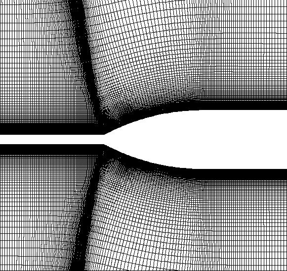
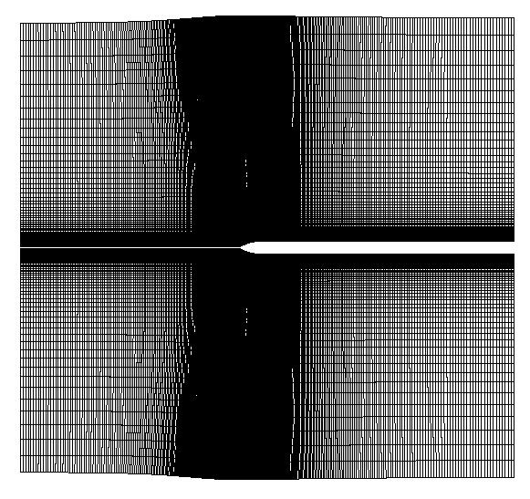
An axisymmetric ogive with the nose tip offsets in the z direction by a given amount is used as an example case. A large nose tip offset, or spacing, represents approximately a 2D case while smaller offsets represent "stronger" axisymmetric cases. The figure of the case when the z offset is 0.1 is shown below. The grid in the z direction was created with two concatenated geometric series. The first series starts at the body, has an initial grid spacing of 1.0E-4, extends out to 0.5, and has 101 points. The second series has an initial grid spacing equal to the final one of the previous series, extends out 20.0, and has 51 points. The second figure below shows a far field view of the grid. The ogive has a radius of 0.5, the nose is 2.0 long, and the cylinder portion of the body is 23 long. As can be seen, the Δr/Δx ratio next to the axis is small.
All the runs in presented in this section are for Euler, Mach=0.3, &alpha=0.0, and &beta=0.0. Slip surface B.C, characteristic outer, inlet, and outlet were used. The section in front of the ogive nose is also slip, i.e. extrapolated density and pressure and normal velocity is set to zero.
The figures below show the average and maximum residual histories for nose offsets of 1000.0, 1.0, 0.1, and 0.01 for the DADI method and 1000.0 and 0.01 for the ADI method. The Beam and Warming ADI method was applied in the &eta direction only. In other words, DADI is always used in the &xi and &zeta direction. The runs shown below were true axisymmetric in the sense there is only one η plane. However, the CFL value is determined based on η planes separated by 5 degrees. The results for the Pulliam Chaussee DADI and Beam Warming ADI methods are identical, to the resolution of the plot, at an offset of 1000.0 and the DADI result is hidden behind the cyan Beam Warming ADI result.
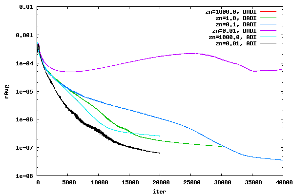
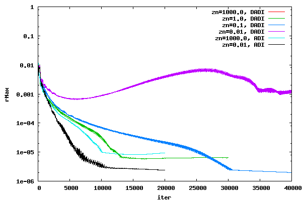
As can be seen in the plots above, as the offset decreases, the DADI solution is unable to converge. On the other hand, as the offset decreases, the ADI converges faster. The faster rate of convergence for ADI for the two offsets could be due to different local time steps or different physics. However, it is clear that DADI and ADI have different trends as the offset decreases. Once the offset gets large, the DADI and ADI method converge to the same residual histories.
Before further cases are run, a test case will be shown comparing axisymmetric and full 3D DADI residual histories for AT CFD. The full 3D case has η planes at every five degrees in the η direction. The axisymmetric case, which solves the case with only one &eta plane, uses a local time step formulation which includes the effects of a η plane at every five degrees. In other words, the axisymmetric and full 3D calculate the time step in exactly the same manner. The intent is to show that the DADI formulation in AT CFD for an axisymmetric case will give the same result as a full 3D case which does not assume axisymmetry. The CFL number was set at 10. The offset was set at 0.01
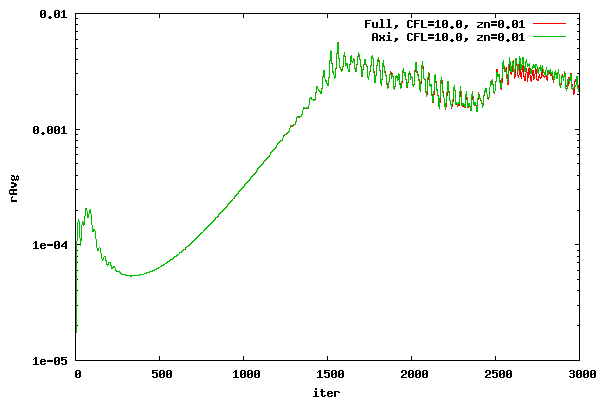
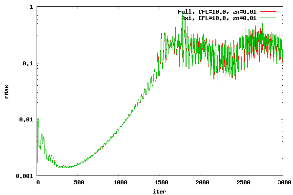
From the plots above, it can be seen that the axisymmetric and 3D DADI methods, as implemented in AT CFD, agree very well. As the number of iterations increase, the two start to diverge due to compounding small differences.
The following plot shows the average residual for a set of CFL runs for a z offset of 0.01, 0.05, and 0.10. The number of iterations has been normalized to represent the convergence for CFL of 10. In other words, the iteration count for the CFL of 2.0 case was multiplied by 2.0/10.0, the CFL of 4.0 case was multiplied by 4.0/10.0, etc. If the residuals were totally time accurate, even in the local time stepping sense, the plots would overlay one another.
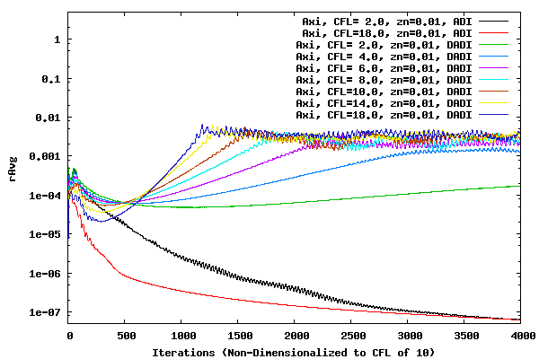
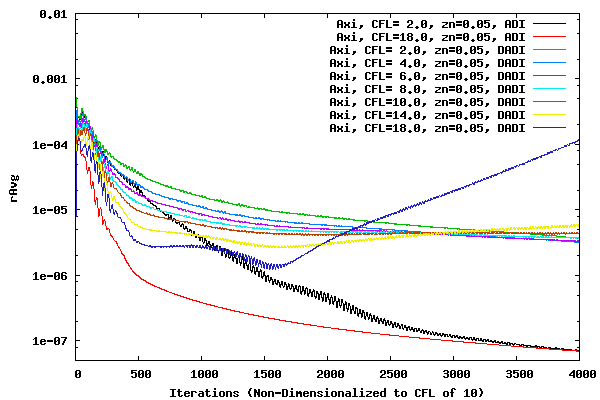
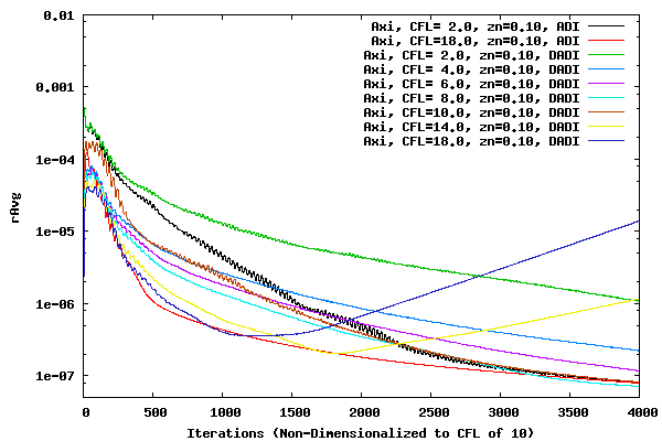
It is interesting to note that the ADI methods with a CFL of 2.0 and 18.0 do not overlay one another until close to 4000 iterations. This could be because of the DADI method being used in the &xi and &zeta direction, or it could be because of loss of time (convergence) accuracy due to large time steps and factorization errors. For all three offset cases above, convergence accuracy decreases with increased CFL number. Therefore, large CFL values can be used to determine the metric value at which the DADI method should switch over to the ADI method. It is also interesting to compare how the offset of 0.10 case loses it's convergence accuracy at higher CFL values to the Vassberg residual history here. It will be interesting at a later date to determine if the divergence of convergence for the Vassberg cases as the CFL number increases is due to the DADI error or the underlying ADI factorization error.
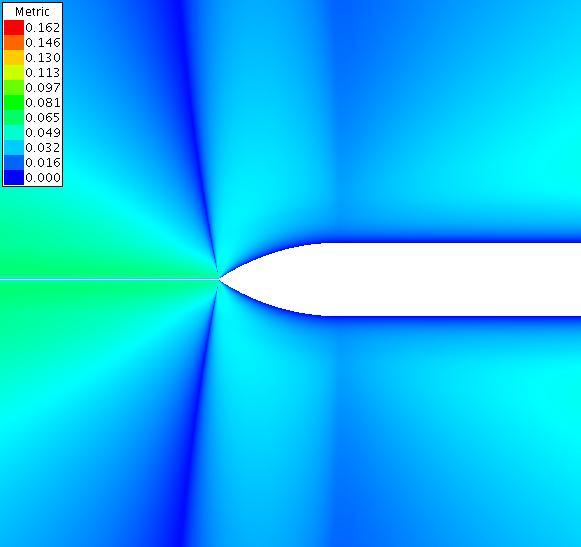
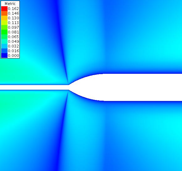
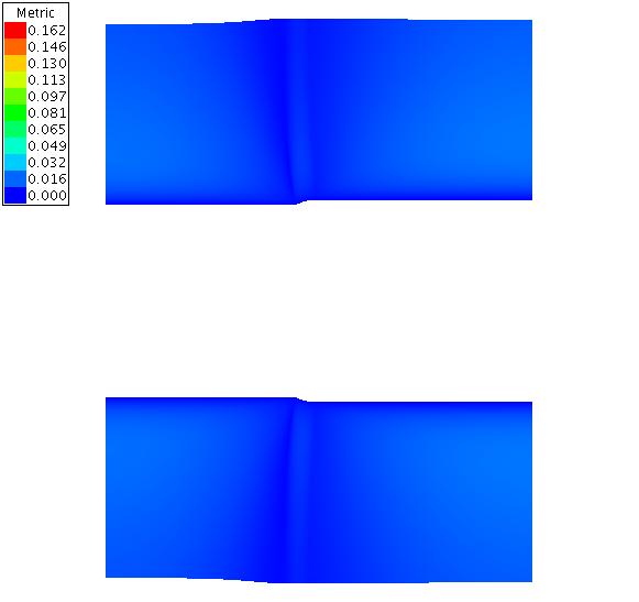
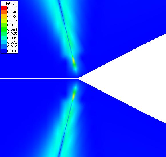
The following contour plots show the metric as calculated by equation 5 for a far and close view of the case with offset 0.00. The contour plots shown below have converged for 4000 iterations at a CFL of 10.0.

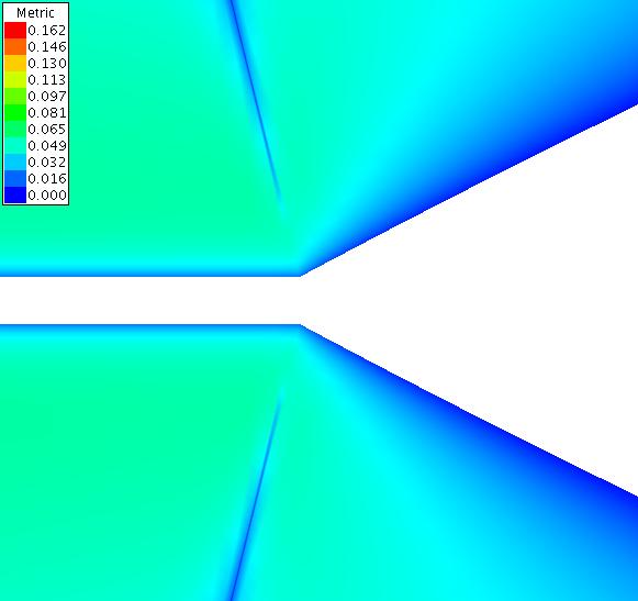
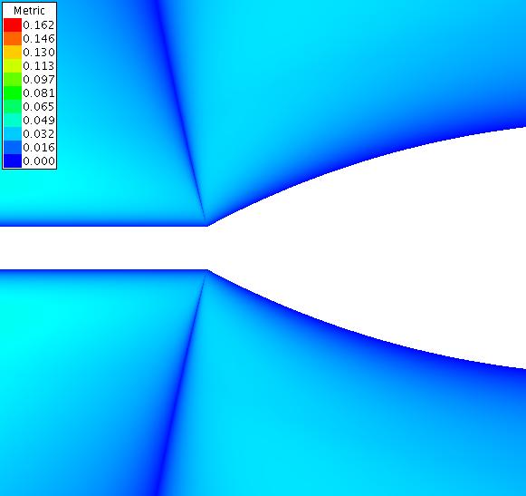
The following contour plots show the metric as calculated by equation 5 for a far and close view of the case with offset 0.01.
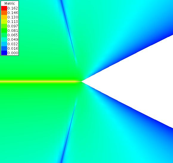
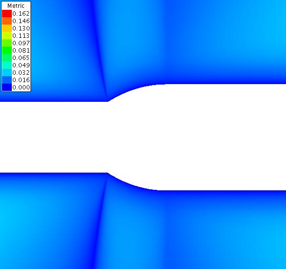
The following contour plots show the metric as calculated by equation 5 for a far and close view of the case with offset 0.10.
The following contour plots show the metric as calculated by equation 5 for a far and close view of the case with offset 1.00.
The following contour plots show the metric as calculated by equation 5 for a far view of the case with offset 10.00.
From the above plots it can be seen that switching over from DADI to ADI at a metric of around 0.05 will probably create a stable convergence history for all cases. Therefore, switch over metric values around 0.05 will be studied to determine convergence behavior. Convergence histories for a range of switch over metrics are shown in the following plots for an offset of 0.00, 0.01, 0.10, and 1.00. A CFL value of 16.0 was used. The switch over metric (met) represents the value at which the DADI switches over to ADI. For example, if the specified switch over metric is 0.05 then any cell with a metric greater than or equal to 0.05 will use ADI and any cell with a metric less than 0.05 will use DADI.
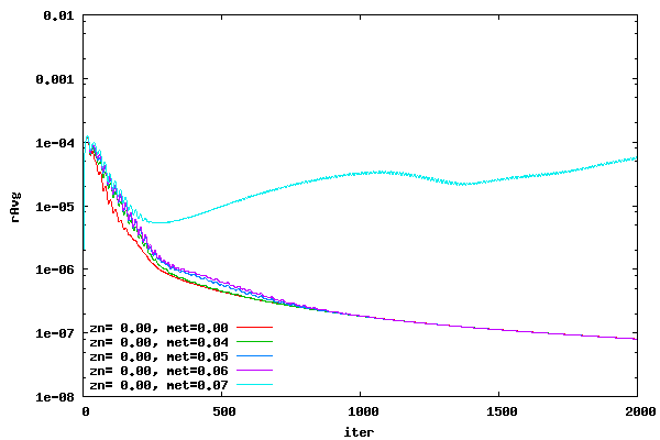
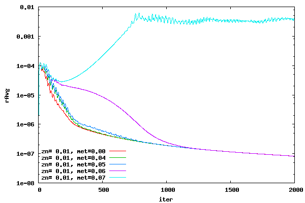
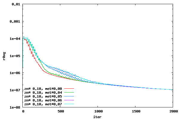
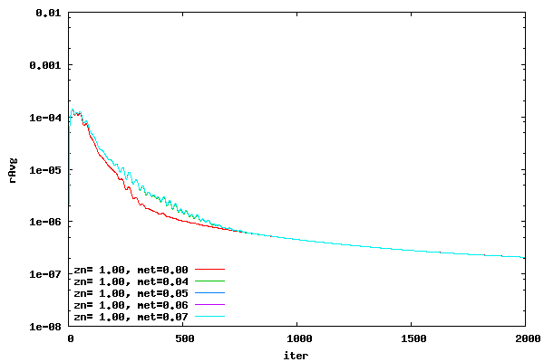
From the plots above it can be seen that a switch over metric of 0.04 creates good convergence histories.
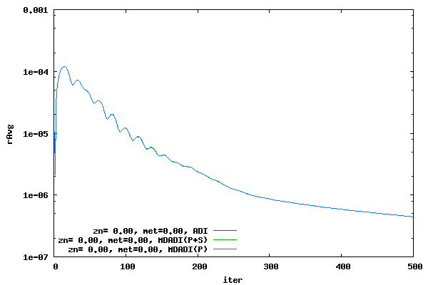
The following two plots compares the MDADI residual history, i.e. traditional DADI method plus equation 3, to the ADI residual history. An offset of 0.00 and a CFL of 16 is used. Plots for the average and maximum residual are shown. Not surprisingly, the MDADI method with the P and S terms is identical to the ADI method. However, what is surprising is that the MDADI with only the P term agrees very well to the ADI method. The reason for this is currently unknown.

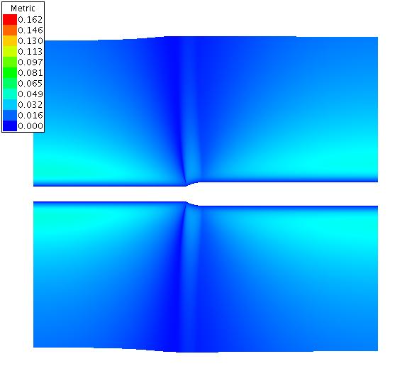
Finally, the plot below is for the metric, as calculated by equation 5, in the ξ direction for zero offset. The plot is a close up of the ogive nose tip. The white strip along the axis is due to the fact that the metric is not calculated on the axis and therefore that portion of the grid is blanked out. The results have converged for 4000 iterations at a CFL of 10.0
Currently, AT CFD does not have the capability to do ADI in the ξ and ζ direction. Therefore, studies involving these directions will need to wait for a later date.
References
1) Pulliam, T. H., and Chaussee, D. S., "A Diagonal Form of an Implicit Approximate-Factorization Algorithm," J. Comput. Phys. 39, 347-363 (1981).
2) Robert H. Nichols, and Pieter G. Buning, "User's Manual for OVERFLOW 2.1," Aug 2008, http://people.nas.nasa.gov/~pulliam/Overflow/Overflow_Manuals.html
Conclusion
A modification to the traditional DADI method was presented to bring DADI back to ADI. The methodology is called MDADI. A metric was presented to assist the CFD user in the determination of when the traditional DADI or the ADI method should be used. This metric can also be used to create a methodology which automatically chooses which portions of the solution space should use DADI and which should use MDADI, in essence creating a methodology which fuses DADI and ADI.