The following example is a CFD analysis and comparison of the decelerator geometry and data presented in
NASA-TM-X-2535 (Ref. 1). The purpose of this example is to demonstrate, to a degree, the effect of eddy viscosity on base drag for a RANS (Spalart Allmaras) CFD solver. Aero Troll CFD was used for this example. Wall functions were not used. Overall, the RANS (SA) solution was able to capture the separation bubble in front of the decelerator but had issues, and uncertainty, with the base pressure.
Description
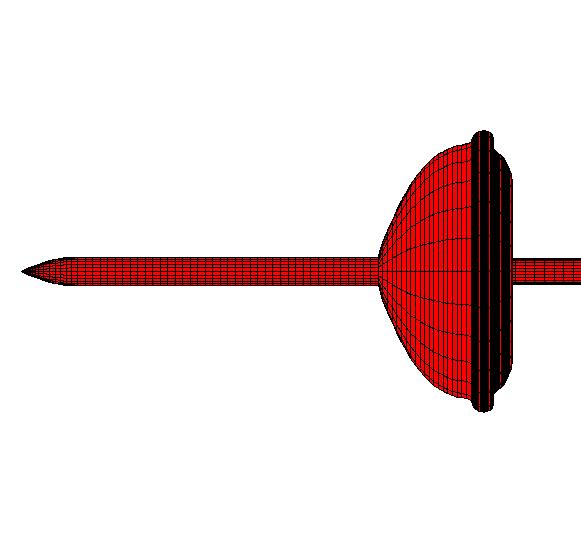
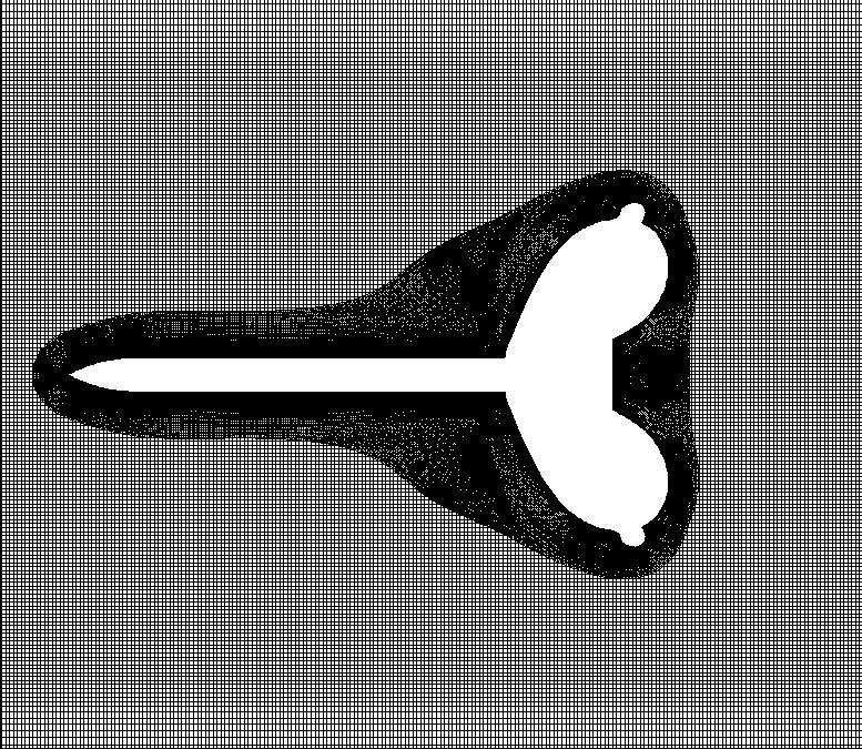
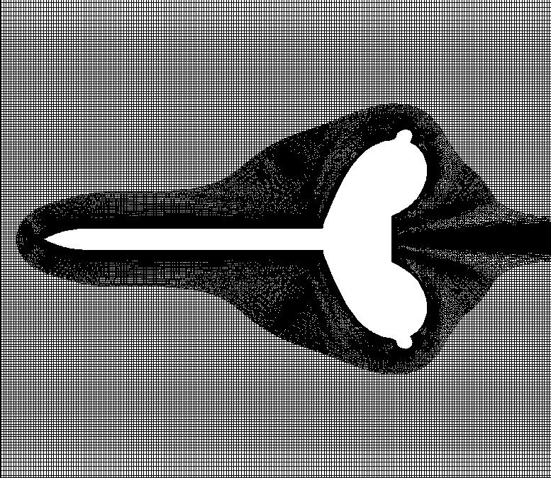
This example is for an inflatable decelerator attached to an ogive-cylinder. The inflatable decelerator was modeled as a solid geometry in the wind tunnel (WT). The WT tests varied in Mach number from Mach 0.20 to 1.00 with corresponding Reynolds numbers of 2.25e6 to 6.90e6 based on the decelerator's diameter (2r
b) at zero angle of attack. For this example, the analysis was made at Mach 0.2 and a Reynolds number of 2.25e6. The decelerator includes a burble fence at the lip of the decelerator and the total max base radius is 1.1 times the decelerator radius (1.1r
b). The figure below shows a representation of the geometry. The decelerator and burble geometry were created by using the pressure tap coordinates given in Reference 1. Since coordinates were not available for corners at the intersections (such as the intersection of the decelerator and burble surfaces), the intersection corner geometry between pressure ports was clipped.
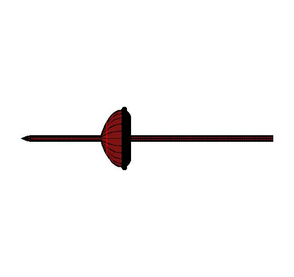
The following view shows the entire geometry.
The ogive nose length is 0.44r
b, the cylinder length is 2.35r
b, and the cylinder radius is 0.11r
b. The sting radius is 0.10r
b. Other than the radius, the sting geometry was not known. Therefore, the length of the sting was made approximately twice the length of the rear flow reattachment length.
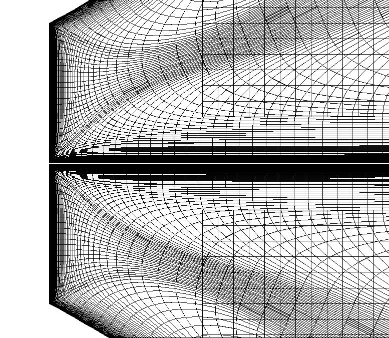
The CFD model was for an axisymmetric geometry. The first off-body grid spacing was at 1.25E-5(rb).
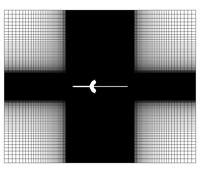
Three different grid sets were used. Each grid set consisted of a body fitted grid imbedded in an axisymmetric cartesian grid. The first grid set is for the body-sting and is shown below.
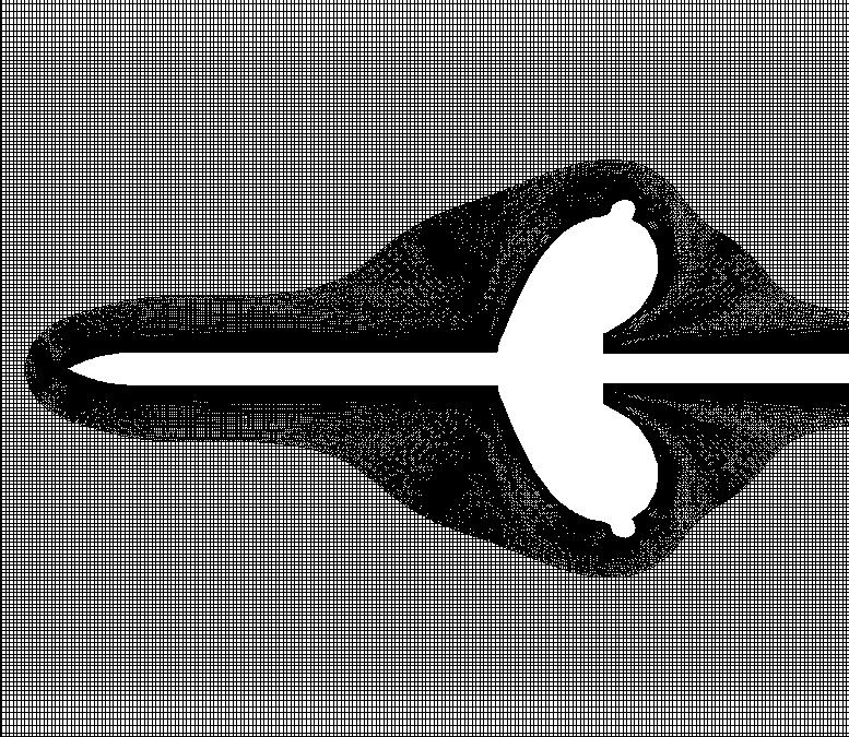
The following image shows the iblanking (cutout) for the axisymmetric cartesian grid.
The following image shows the far field. Note that the far field is only about 12r
b away. For a rigorous analysis the far field should be changed to around 50r
b.
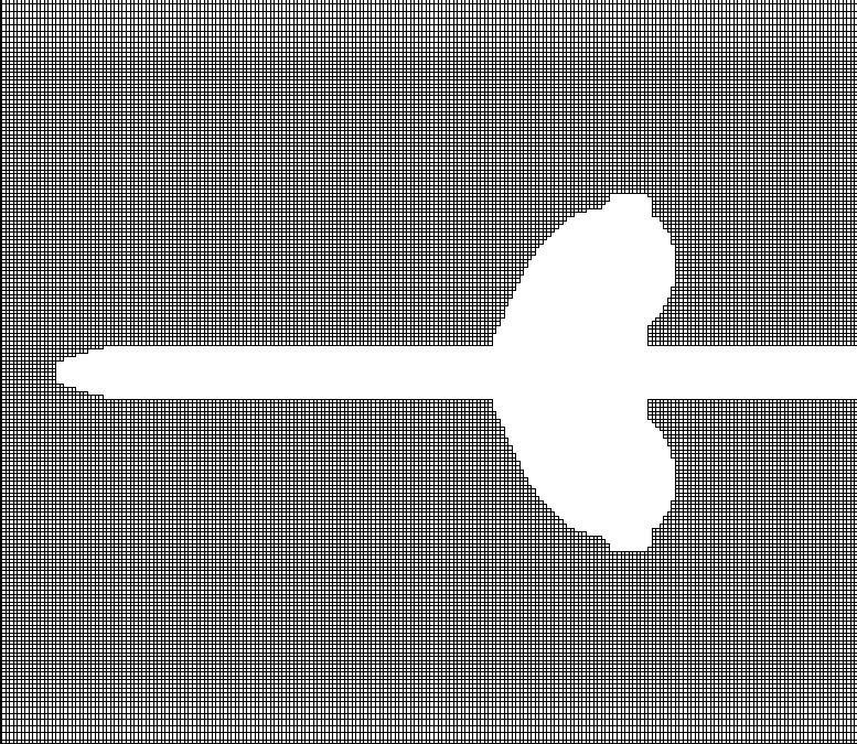
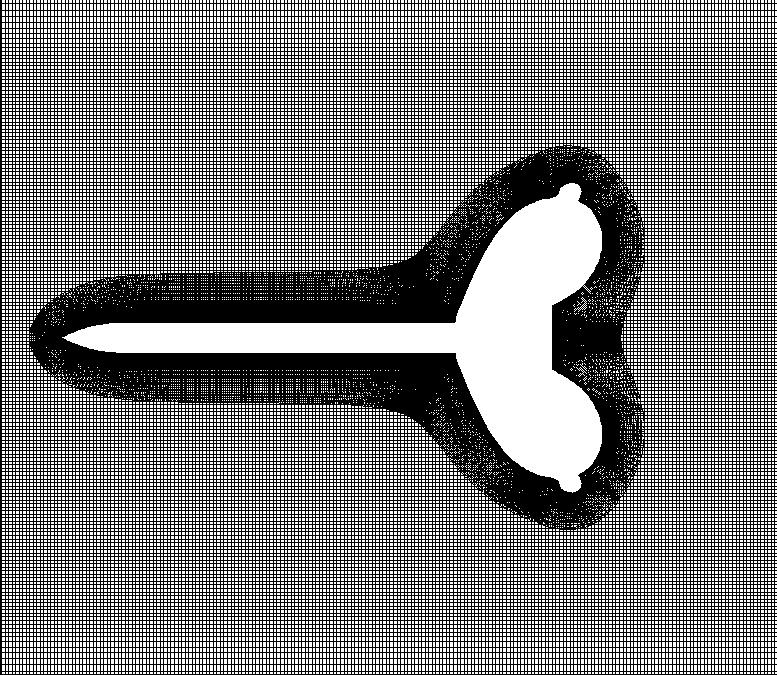
The second grid set is for the body alone.
The third grid set is for the body alone using a slightly different hyperbolic grid generation setting to alter the body fitted grid.
Results
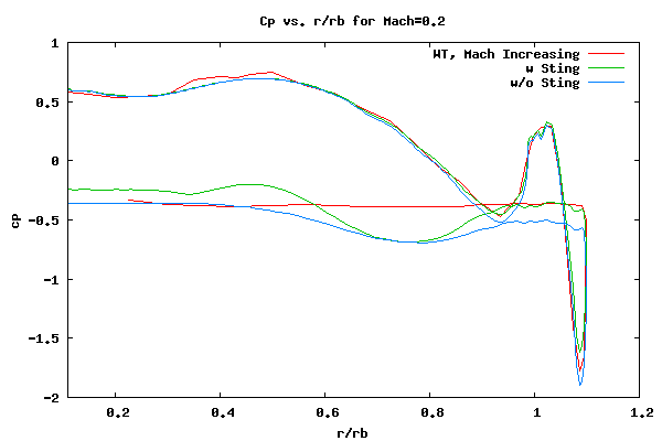
The pressure coefficient comparison vs. r/r
b for the data and various CFD results are shown below. The cp plot shows two curves for the experimental Mach 0.2 results. One data sampling was taken at Mach 0.2 when the Mach number was increased to Mach 1.0 and the other was taken when the the Mach number was decreased from Mach 1.0. The front side data and CFD results are, on average, the high pressure portion of the curve and the backside is the low pressure portion.
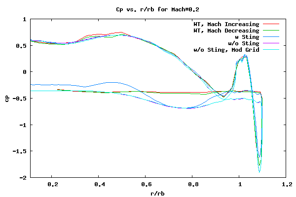
The above plot shows that the CFD compares relatively well to data for the front side of the decelerator and burble. The no-sting results with the original and modified grid are very close to one another so the two are hard to differentiate. The CFD is able to capture the separation bubble in front of the decelerator. The results without a sting are slightly off from the data in the region before the burble. The result with a sting agree well. Both the no-sting and sting data are slightly off along the top of the burble. This could because of difficulty in capturing the boundary layer profile after the reattachment of the forward separation bubble. This is to be expected. Or it could be because of gridding. Further investigation is required at a later date.
The back side is somewhat of a different story. The cp values for the backside data are mostly constant, and this is expected. On the other hand, the sting and no-sting CFD results show a significant difference between one another and, overall, neither have the same qualitative trend that the WT data has. It seems that the sting data agrees better with the no-sting results, especially at the outer region. The following plot shows a cleaned up version of the above plot. Only the increasing data, sting, and no-sting data on the unmodified grid is shown.
When one looks at the above grid, it seems that the sting CFD agrees better than the no-sting data. This is great news since the WT geometry has a sting! However, caution must be exercised since, in general, the addition of a sting should not have too much influence on the base pressure. The backside of the decelerator is a dead air region. To investigate this thoroughly, and try not to jump to conclusions about trends for real world no-sting data, another run was made with a very thin sting. The following images show a followup case where the sting radius was set to 0.001r
b.
A closeup view of the base is shown below.
The results with the wire sting is shown below.
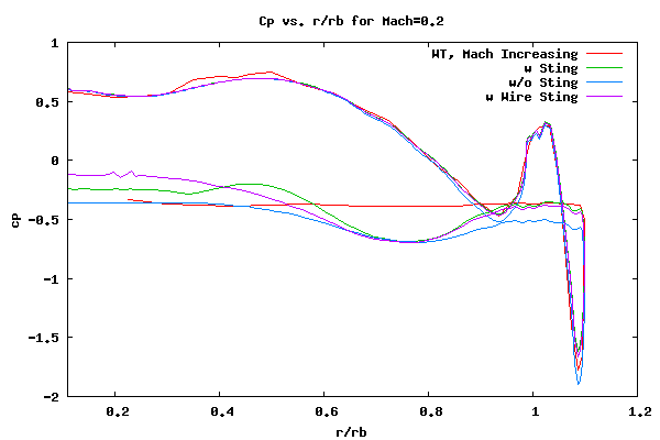
As can be seen from the above plot, the wire-sting and no-sting do not compare well close to the center line. To understand the difference, the eddy viscosity plots need to be looked at. The eddy viscosity plots for the no-sting, sting, and wire-sting are shown below.
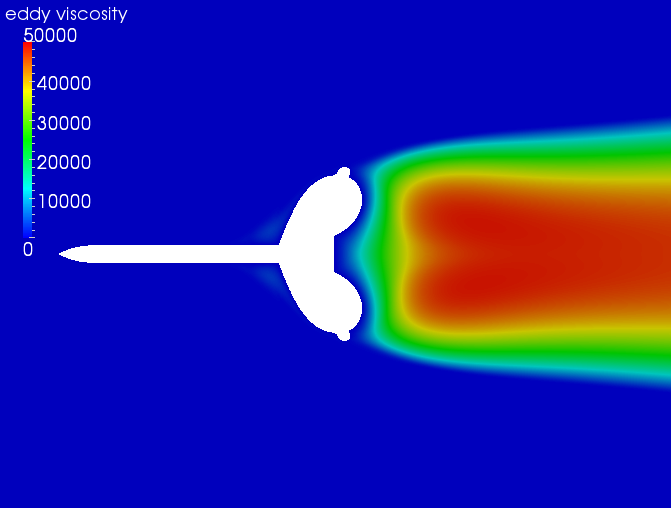
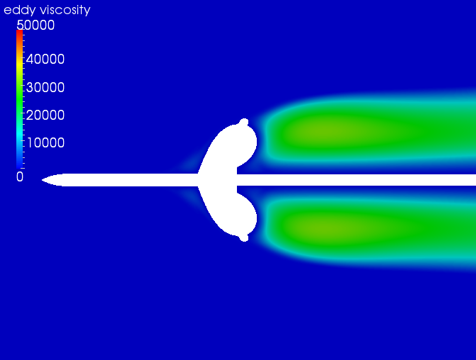
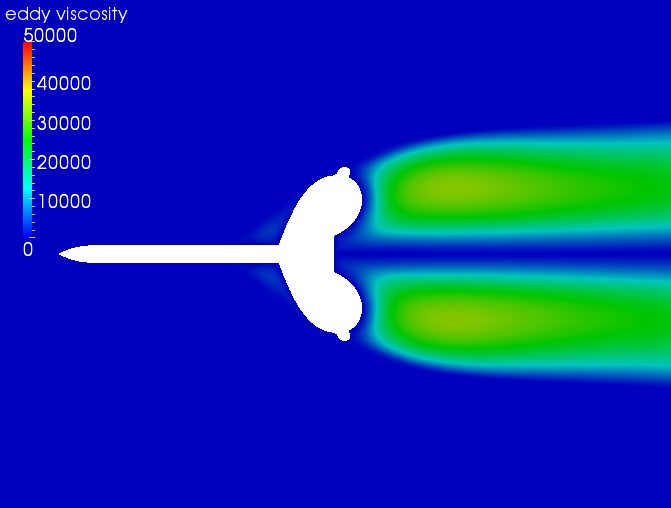
As can be seen in the plot above, the eddy viscosity for the wire-sting and no-sting geometries are very different. The overall lower values for the wire sting are due to the boundary condition requirement that the eddy viscosity on a surface (i.e. the wire sting) must be zero. The lower eddy viscosity values for the sting and wire-sting geometries are probably why the pressure on the backside of the burble agree well. However, overall, one may not be able to say which CFD result is "better" since the eddy viscosity RANS model does not really capture the nuances of the physics. Caution must be exercised!
References
1) Sawyer, J. W., "
Subsonic pressure distributions around a solid model of an inflatable decelerator attached to the base of an ogive-cylinder," NASA-TM-X-2535, Apr 1, 1972.